Accelerate Sentence Transformers with Hugging Face Optimum
last update: 2022-11-18
In this session, you will learn how to optimize Sentence Transformers using Optimum. The session will show you how to dynamically quantize and optimize a MiniLM Sentence Transformers model using Hugging Face Optimum and ONNX Runtime. Hugging Face Optimum is an extension of 🤗 Transformers, providing a set of performance optimization tools enabling maximum efficiency to train and run models on targeted hardware.
Note: dynamic quantization is currently only supported for CPUs, so we will not be utilizing GPUs / CUDA in this session.
By the end of this session, you see how quantization and optimization with Hugging Face Optimum can result in significant decrease in model latency.
You will learn how to:
- Setup Development Environment
- Convert a Sentence Transformers model to ONNX and create custom Inference Pipeline
- Apply graph optimization techniques to the ONNX model
- Apply dynamic quantization using
ORTQuantizerfrom Optimum - Test inference with the quantized model
- Evaluate the performance and speed
Let's get started! 🚀
This tutorial was created and run on an c6i.xlarge AWS EC2 Instance.
Quick intro: What are Sentence Transformers
Sentence Transformers is a Python library for state-of-the-art sentence, text and image embeddings. The initial work is described in our paper Sentence-BERT: Sentence Embeddings using Siamese BERT-Networks.
Sentence Transformers can be used to compute embeddings for more than 100 languages and to build solutions for semantic textual similar, semantic search, or paraphrase mining.
1. Setup Development Environment
Our first step is to install Optimum, along with Evaluate and some other libraries. Running the following cell will install all the required packages for us including Transformers, PyTorch, and ONNX Runtime utilities:
!pip install "optimum[onnxruntime]==1.5.0" transformers evaluate mkl-include mkl --upgradeIf you want to run inference on a GPU, you can install 🤗 Optimum with
pip install optimum[onnxruntime-gpu].
2. Convert a Sentence Transformers model to ONNX and create custom Inference Pipeline
Before we can start qunatizing we need to convert our vanilla sentence-transformers model to the onnx format. To do this we will use the new ORTModelForFeatureExtraction class calling the from_pretrained() method with the from_transformers attribute. The model we are using is the sentence-transformers/all-MiniLM-L6-v2 which maps sentences & paragraphs to a 384 dimensional dense vector space and can be used for tasks like clustering or semantic search and was trained on the 1-billion sentence dataset.
from optimum.onnxruntime import ORTModelForFeatureExtraction
from transformers import AutoTokenizer
from pathlib import Path


model_id="sentence-transformers/all-MiniLM-L6-v2"
onnx_path = Path("onnx")

# load vanilla transformers and convert to onnx
model = ORTModelForFeatureExtraction.from_pretrained(model_id, from_transformers=True)
tokenizer = AutoTokenizer.from_pretrained(model_id)

# save onnx checkpoint and tokenizer
model.save_pretrained(onnx_path)
tokenizer.save_pretrained(onnx_path)
When using sentence-transformers natively you can run inference by loading your model in the SentenceTransformer class and then calling the .encode() method. However this only works with the PyTorch based checkpoints, which we no longer have. To run inference using the Optimum ORTModelForFeatureExtraction class, we need to write some methods ourselves. Below we create a SentenceEmbeddingPipeline based on "How to create a custom pipeline?" from the Transformers documentation.
from transformers import Pipeline
import torch.nn.functional as F
import torch

# copied from the model card
def mean_pooling(model_output, attention_mask):
    token_embeddings = model_output[0] #First element of model_output contains all token embeddings
    input_mask_expanded = attention_mask.unsqueeze(-1).expand(token_embeddings.size()).float()
    return torch.sum(token_embeddings * input_mask_expanded, 1) / torch.clamp(input_mask_expanded.sum(1), min=1e-9)


class SentenceEmbeddingPipeline(Pipeline):
    def _sanitize_parameters(self, **kwargs):
        # we don't have any hyperameters to sanitize
        preprocess_kwargs = {}
        return preprocess_kwargs, {}, {}

    def preprocess(self, inputs):
        encoded_inputs = self.tokenizer(inputs, padding=True, truncation=True, return_tensors='pt')
        return encoded_inputs

    def _forward(self, model_inputs):
        outputs = self.model(**model_inputs)
        return {"outputs": outputs, "attention_mask": model_inputs["attention_mask"]}

    def postprocess(self, model_outputs):
        # Perform pooling
        sentence_embeddings = mean_pooling(model_outputs["outputs"], model_outputs['attention_mask'])
        # Normalize embeddings
        sentence_embeddings = F.normalize(sentence_embeddings, p=2, dim=1)
        return sentence_embeddings
We can now initialize our SentenceEmbeddingPipeline using our ORTModelForFeatureExtraction model and perform inference.
# init pipeline
vanilla_emb = SentenceEmbeddingPipeline(model=model, tokenizer=tokenizer)

# run inference
pred = vanilla_emb("Could you assist me in finding my lost card?")

# print an excerpt from the sentence embedding
print(pred[0][:5])
#     tensor([-0.0631,  0.0426,  0.0037,  0.0377,  0.0414])
If you want to learn more about exporting transformers model check-out Convert Transformers to ONNX with Hugging Face Optimum blog post
3. Apply graph optimization techniques to the ONNX model
Graph optimizations are essentially graph-level transformations, ranging from small graph simplifications and node eliminations to more complex node fusions and layout optimizations. Examples of graph optimizations include:
- Constant folding: evaluate constant expressions at compile time instead of runtime
- Redundant node elimination: remove redundant nodes without changing graph structure
- Operator fusion: merge one node (i.e. operator) into another so they can be executed together
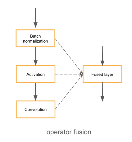
If you want to learn more about graph optimization you take a look at the ONNX Runtime documentation. We are going to first optimize the model and then dynamically quantize to be able to use transformers specific operators such as QAttention for quantization of attention layers.
To apply graph optimizations to our ONNX model, we will use the ORTOptimizer(). The ORTOptimizer makes it with the help of a OptimizationConfig easy to optimize. The OptimizationConfig is the configuration class handling all the ONNX Runtime optimization parameters.
from optimum.onnxruntime import ORTOptimizer
from optimum.onnxruntime.configuration import OptimizationConfig

# create ORTOptimizer and define optimization configuration
optimizer = ORTOptimizer.from_pretrained(model)
optimization_config = OptimizationConfig(optimization_level=99) # enable all optimizations

# apply the optimization configuration to the model
optimizer.optimize(
    save_dir=onnx_path,
    optimization_config=optimization_config,
)
To test performance we can use the ORTModelForSequenceClassification class again and provide an additional file_name parameter to load our optimized model. (This also works for models available on the hub).
from optimum.onnxruntime import ORTModelForFeatureExtraction

# load optimized model
model = ORTModelForFeatureExtraction.from_pretrained(onnx_path, file_name="model_optimized.onnx")

# create optimized pipeline
optimized_emb = SentenceEmbeddingPipeline(model=model, tokenizer=tokenizer)
pred = optimized_emb("Could you assist me in finding my lost card?")
print(pred[0][:5])
#  tensor([-0.0631,  0.0426,  0.0037,  0.0377,  0.0414])
4. Apply dynamic quantization using ORTQuantizer from Optimum
After we have optimized our model we can accelerate it even more by quantizing it using the ORTQuantizer. The ORTQuantizer can be used to apply dynamic quantization to decrease the size of the model size and accelerate latency and inference.
We use the avx512_vnni config since the instance is powered by an intel ice-lake CPU supporting avx512.
from optimum.onnxruntime import ORTQuantizer
from optimum.onnxruntime.configuration import AutoQuantizationConfig

# create ORTQuantizer and define quantization configuration
dynamic_quantizer = ORTQuantizer.from_pretrained(model)
dqconfig = AutoQuantizationConfig.avx512_vnni(is_static=False, per_channel=False)

# apply the quantization configuration to the model
model_quantized_path = dynamic_quantizer.quantize(
    save_dir=onnx_path,
    quantization_config=dqconfig,
)
Lets quickly check the new model size.
import os

# get model file size
size = os.path.getsize(onnx_path / "model_optimized.onnx")/(1024*1024)
quantized_model = os.path.getsize(onnx_path / "model_optimized_quantized.onnx")/(1024*1024)

print(f"Model file size: {size:.2f} MB")
print(f"Quantized Model file size: {quantized_model:.2f} MB")
#  Model file size: 86.66 MB
#  Quantized Model file size: 63.47 MB
5. Test inference with the quantized model
Optimum has built-in support for transformers pipelines. This allows us to leverage the same API that we know from using PyTorch and TensorFlow models.
Therefore we can load our quantized model with ORTModelForSequenceClassification class and transformers pipeline.
from optimum.onnxruntime import ORTModelForFeatureExtraction
from transformers import AutoTokenizer

model = ORTModelForFeatureExtraction.from_pretrained(onnx_path,file_name="model-quantized.onnx")
tokenizer = AutoTokenizer.from_pretrained(onnx_path)

q8_emb = SentenceEmbeddingPipeline(model=model, tokenizer=tokenizer)

pred = q8_emb("Could you assist me in finding my lost card?")
print(pred[0][:5])
# tensor([-0.0567,  0.0111, -0.0110,  0.0450,  0.0447])
6. Evaluate the performance and speed
As the last step, we want to take a detailed look at the performance and accuracy of our model. Applying optimization techniques, like graph optimizations or mixed-precision not only impact performance (latency) those also might have an impact on the accuracy of the model. So accelerating your model comes with a trade-off.
We are going to evaluate our Sentence Transformers model / Sentence Embeddings on the Semantic Textual Similarity Benchmark from the GLUE dataset.
The Semantic Textual Similarity Benchmark (Cer et al., 2017) is a collection of sentence pairs drawn from news headlines, video and image captions, and natural language inference data. Each pair is human-annotated with a similarity score from 1 to 5.
from datasets import load_dataset
from evaluate import load

eval_dataset = load_dataset("glue","stsb",split="validation")
metric = load('glue', 'stsb')

# creating a subset for faster evaluation
# COMMENT IN to run evaluation on a subset of the dataset
# eval_dataset = eval_dataset.select(range(200))
We can now leverage the map function of datasets to iterate over the validation set of stsb and run prediction for each data point. Therefore we write a evaluate helper method which uses our SentenceEmbeddingsPipeline and sentence-transformers helper methods.
def compute_sentence_similarity(sentence_1, sentence_2,pipeline):
    embedding_1 = pipeline(sentence_1)
    embedding_2 = pipeline(sentence_2)
    # compute cosine similarity between two sentences
    return torch.nn.functional.cosine_similarity(embedding_1, embedding_2, dim=1)


def evaluate_stsb(example):
  default = compute_sentence_similarity(example["sentence1"], example["sentence2"], vanilla_emb)
  quantized = compute_sentence_similarity(example["sentence1"], example["sentence2"], q8_emb)
  return {
      'reference': (example["label"] - 1) / (5 - 1), # rescale to [0,1]
      'default': float(default),
      'quantized': float(quantized),
      }

# run evaluation
result = eval_dataset.map(evaluate_stsb)

# compute metrics
default_acc = metric.compute(predictions=result["default"], references=result["reference"])
quantized = metric.compute(predictions=result["quantized"], references=result["reference"])

print(f"vanilla model: pearson={default_acc['pearson']}%")
print(f"quantized model: pearson={quantized['pearson']}%")
print(f"The quantized model achieves {round(quantized['pearson']/default_acc['pearson'],2)*100:.2f}% accuracy of the fp32 model")
the results are
vanilla model: pearson=0.8696194595133899%
quantized model: pearson=0.8663752613975557%
The quantized model achieves 100.00% accuracy of the fp32 model
Okay, now let's test the performance (latency) of our quantized model. We are going to use a payload with a sequence length of 128 for the benchmark. To keep it simple, we are going to use a python loop and calculate the avg,mean & p95 latency for our vanilla model and for the quantized model.
from time import perf_counter
import numpy as np
payload="Hello, my name is Philipp and I live in Nuremberg, Germany. Currently I am working as a Technical Lead at Hugging Face to democratize artificial intelligence through open source and open science. In the past I designed and implemented cloud-native machine learning architectures for fin-tech and insurance companies. I found my passion for cloud concepts and machine learning 5 years ago. Since then I never stopped learning. Currently, I am focusing myself in the area NLP and how to leverage models like BERT, Roberta, T5, ViT, and GPT2 to generate business value. I cannot wait to see what is next for me"
print(f'Payload sequence length: {len(tokenizer(payload)["input_ids"])}')
def measure_latency(pipe):
latencies = []
# warm up
for _ in range(10):
_ = pipe(payload)
# Timed run
for _ in range(100):
start_time = perf_counter()
_ = pipe(payload)
latency = perf_counter() - start_time
latencies.append(latency)
# Compute run statistics
time_avg_ms = 1000 * np.mean(latencies)
time_std_ms = 1000 * np.std(latencies)
time_p95_ms = 1000 * np.percentile(latencies,95)
return f"P95 latency (ms) - {time_p95_ms}; Average latency (ms) - {time_avg_ms:.2f} +\- {time_std_ms:.2f};", time_p95_ms
vanilla_model=measure_latency(vanilla_emb)
quantized_model=measure_latency(q8_emb)
print(f"Vanilla model: {vanilla_model[0]}")
print(f"Quantized model: {quantized_model[0]}")
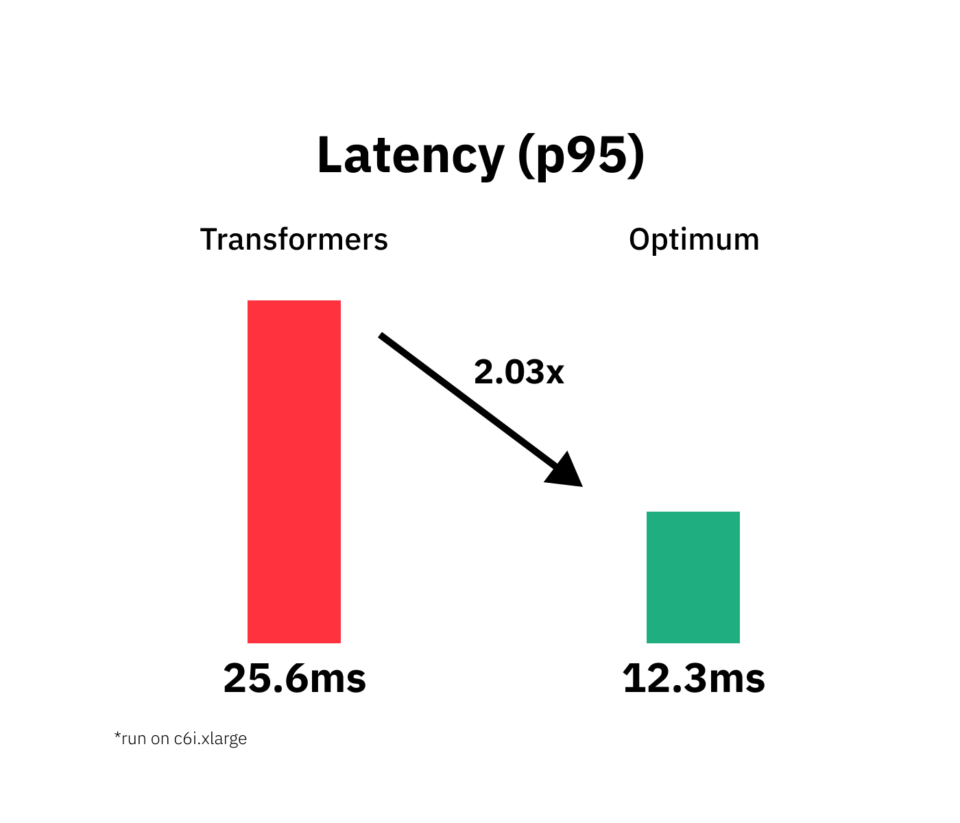
print(f"Improvement through quantization: {round(vanilla_model[1]/quantized_model[1],2)}x")the results are
Payload sequence length: 128
Vanilla model: P95 latency (ms) - 25.639022301038494; Average latency (ms) - 19.75 +\- 2.72;
Quantized model: P95 latency (ms) - 12.289083890937036; Average latency (ms) - 11.76 +\- 0.37;
Improvement through quantization: 2.09x
We managed to accelerate our model latency from 25.6ms to 12.3ms or 2.09x while keeping 100% of the accuracy on the stsb dataset.
Conclusion
We successfully quantized our vanilla Transformers model with Hugging Face and managed to accelerate our model latency from 25.6ms to 12.3ms or 2.09x while keeping 100% of the accuracy on the stsb dataset.
But I have to say that this isn't a plug and play process you can transfer to any Transformers model, task or dataset.