Getting Started with AutoML and AWS AutoGluon
Google CEO Sundar Pichai wrote, “... designing neural nets is extremely time intensive, and requires an expertise that limits its use to a smaller community of scientists and engineers." Shortly after this Google launched its service AutoML in early 2018.
AutoML aims to enable developers with limited machine learning expertise to train high-quality models specific to their business needs. The goal of AutoML is to automate all the major repetitive tasks such as feature selection or hyperparameter tuning. This allows creating more models in less time with improved quality and accuracy.
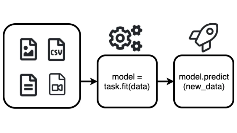
A basic two step approach to machine learning: First, the model is created by fitting it to the data. Second, the model is used to predict the output for new (previously unseen) data.
This blog post demonstrates how to get started quickly with AutoML. It will give you a step-by-step tutorial on how to built an Object Detection Model using AutoGluon, with top-notch accuracy. I created a Google Colab Notebook with a full example.
AWS is entering the field of AutoML
At Re:Invent 2019 AWS launched a bunch on add-ons for there managed machine Learning service Sagemaker amongst other "Sagemaker Autopilot". Sagemaker Autopilot is an AutoML Service comparable to Google AutoML service.
In January 2020 Amazon Web Services Inc. (AWS) secretly launched an open-source library called AutoGluon the library behind Sagemaker Autopilot.
AutoGluon enables developers to write machine learning-based applications that use image, text or tabular data sets with just a few lines of code.

With those tools, AWS has entered the field of managed AutoML Services or MLaas and to compete Google with its AutoML service.
What is AutoGluon?
"AutoGluon enables easy-to-use and easy-to-extend AutoML with a focus on deep learning and real-world applications spanning image, text, or tabular data. Intended for both ML beginners and experts, AutoGluon enables you to... "
- quickly prototype deep learning solutions
- automatic hyperparameter tuning, model selection / architecture search
- improve existing bespoke models and data pipelines **
AutoGluon enables you to build machine learning models with only 3 Lines of Code.
from autogluon import TabularPrediction as task

predictor = task.fit(train_data=task.Dataset(file_path="TRAIN_DATA.csv"), label="PREDICT_COLUMN")
predictions = predictor.predict(task.Dataset(file_path="TEST_DATA.csv"))
Currently, AutoGluon can create models for image classification, object detection, text classification, and supervised learning with tabular datasets.
If you are interested in how AutoGluon is doing all the magic behind the scenes take a look at the "Machine learning with AutoGluon, an open source AutoML library" Post on the AWS Open Source Blog.
Tutorial
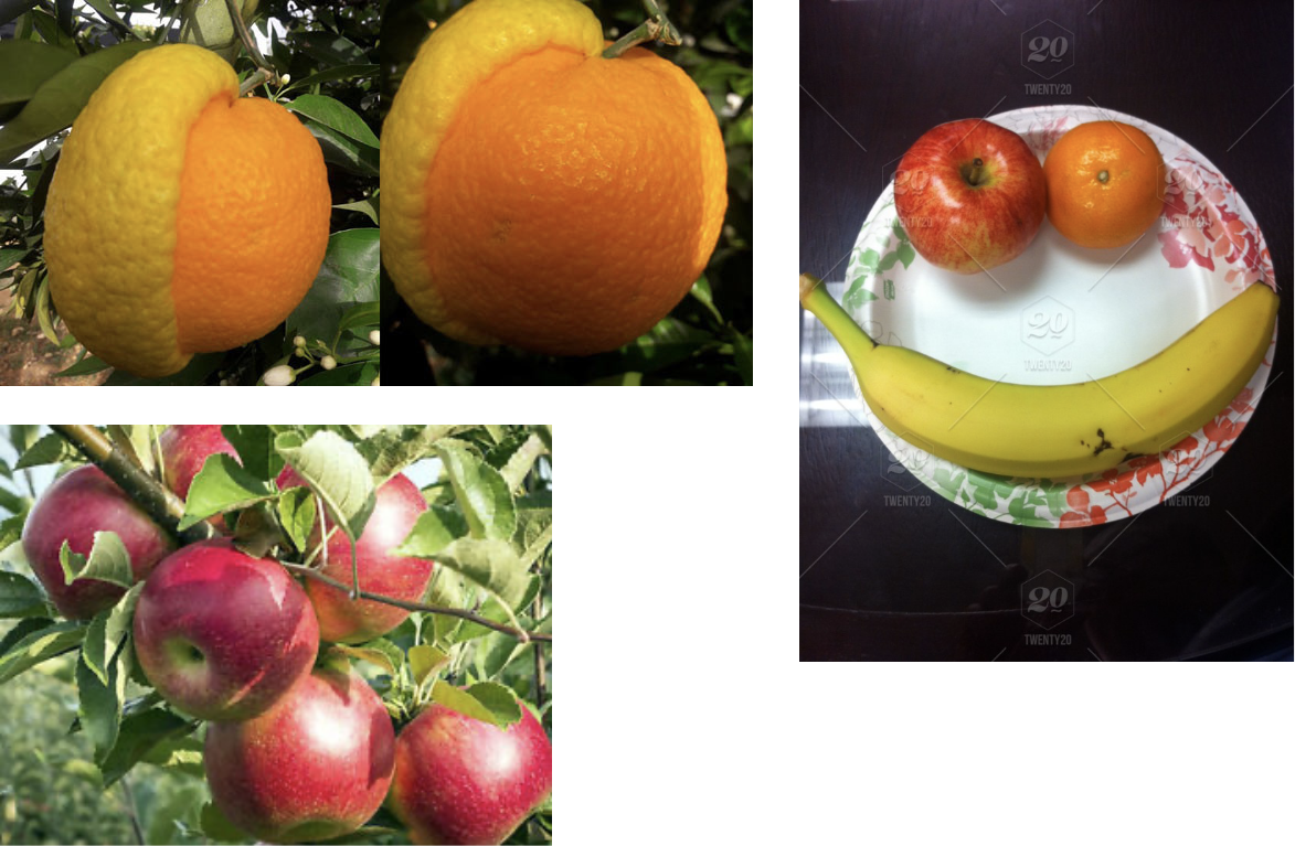
We are going to build an Object Detection Model, to detect fruits (apple, orange and banana) on images. I built a small dataset with around 300 images to achieve a quick training process. You can find the dataset here.
I am using Google Colab with a GPU runtime for this tutorial. If you are not sure how to use a GPU Runtime take a look here.
Okay, now let's get started with the tutorial.
Installing AutoGluon
AutoGluon offers different installation packages for different hardware preferences. For more installation instructions take a look at the AutoGluon Installation Guide here.
The first step is to install AutoGluon with pip and CUDA support.
# Here we assume CUDA 10.0 is installed.  You should change the number
# according to your own CUDA version (e.g. mxnet-cu101 for CUDA 10.1).
!pip install --upgrade mxnet-cu100
!pip install autogluon
For AutoGluon to work in Google Colab, we also have to install ipykernel and restart the runtime.
!pip install -U ipykernelAfter a successful restart of your runtime you can import autogluon and print out the version.
import autogluon as ag
from autogluon import ObjectDetection as task

print(ag.__version__)

# >>>> '0.0.6'
Loading data and creating datasets
The next step is to load the dataset we use for the object detection task. In the ObjectDetection task from AutoGluon,
you can either use PASCAL VOC format or the COCO format by adjusting the format parameter of Dataset() to either
coco or voc. The
Pascal VOC Dataset contains
two directories: Annotations and JPEGImages. The
COCO dataset is
formatted in JSON and is a collection of "info", "licenses", "images", "annotations", "categories".
For training, we are going to use the tiny_fruit_object_detection dataset, which I build. The Dataset contains around 300 images of bananas, apples, oranges or a combination of them together.
We are using 240 images for training, 30 for testing and 30 for evaluating the model.
Using the commands below, we can download and unzip this dataset, which is only 29MB. After this we create our
Dataset for train and test with task.Dataset().
# download the data
root = './'
filename_zip = ag.download('https://philschmid-datasets.s3.eu-central-1.amazonaws.com/tiny_fruit.zip',
                        path=root)
# unzip data
filename = ag.unzip(filename_zip, root=root)

# create Dataset
data_root = os.path.join(root, filename)
# train dataset
dataset_train = task.Dataset(data_root, classes=('banana','apple','orange'),format='voc')
# test dataset
dataset_test = task.Dataset(data_root, index_file_name='test', classes=('banana','apple','orange'),format='voc')
Training the Model
The third step is to train our model with the created dataset. In AutoGluon you define your classifier as variable,
here detector and define parameters in the fit() function during train-time. For example, you can define a
time_limit which automatically stops the training after a certain time. You can define a range for your own
learning_rate or set the number of epochs. One of the most important parameters is num_trials. This parameter
defines the maximum number of hyperparameter configurations to try out. You can find the full documentation of the
configurable parameters here.
We are going to train our model for 20 epochs and train 3 different models by setting num_trials=3.
from autogluon import ObjectDetection as task
epochs = 20
detector = task.fit(dataset_train,
num_trials=3,
epochs=epochs,
lr=ag.Categorical(5e-4, 1e-4, 3e-4),
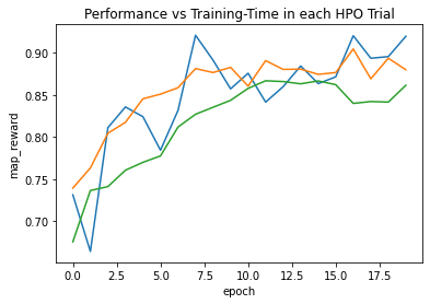
ngpus_per_trial=1)As a result, we are getting a chart with the mean average precision (mAP) and the number of epochs. The mAP is a common metric to calculate the accuracy of an object detection model.
Our best model (blue-line) achieved an mAP of 0.9198171507070327
Evaluating the Model
After finishing training, we are now going to evaluate/test the performance of our model on our test dataset
test_map = detector.evaluate(dataset_test)
print(f"The mAP on the test dataset is {test_map[1][1]}")
The mAP on the test dataset is 0.8724113724113725 which is pretty good considering we only training with 240 Images
and 20 epochs.
Predict an Image
To use our trained model for predicting you can simply run detector.predict(image_path), which will return a tuple
(ind) containing the class-IDs of detected objects, the confidence-scores (prob), and the corresponding predicted
bounding box locations (loc).
image = 'mixed_10.jpg'
image_path = os.path.join(data_root, 'JPEGImages', image)

ind, prob, loc = detector.predict(image_path)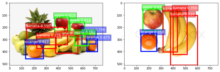
Save Model
As of the time writing this article, saving an object detection model is not yet implemented in version 0.0.6, but
will be in the next deployed version.
To save your model, you only have to run detector.save()
savefile = 'model.pkl'
detector.save(savefile)
Load Model
As of the time writing this article, loading an object detection model is not yet implemented in version 0.0.6, but
will be in the next deployed version.
from autogluon import Detector
new_detector = Detector.load(savefile)

image = 'mixed_17.jpg'
image_path = os.path.join(data_root, 'JPEGImages', image)

detector.predict(image_path)
Thanks for reading. You can find the Google Colab Notebook containing a full example here.